non-equi merge in data.table and epidemiology
How to use non-equi merges to solve common problems of data management in epidemiology
The idea of this post is to explain and show example of use of non equi join in data.table. I use a lot this feature, which I find incredibly usefull.
Some basic ideas of data.table
library(data.table)
library(lubridate)
library(ggplot2)
library(magrittr)
I recommend this vignette for those who do not know data.table. The basic ideas you need for this post:
df <- data.table(a = rep(c(1:4),each = 2),x = sample(letters,4))
df
## a x
## 1: 1 d
## 2: 1 t
## 3: 2 h
## 4: 2 m
## 5: 3 d
## 6: 3 t
## 7: 4 h
## 8: 4 mThere are 3 parts in a data.table:
df[i,j,k]i is to subset the data.table, j to do operation on the columns, and k to do grouping operations.
You assign value to a new variable using :=:
df[,y := 1:8]When you subset a value, you can subset on a variable value:
df[a == 1]## a x y
## 1: 1 d 1
## 2: 1 t 2or you can use an other data.table. For example if I consider a second data.table
df2 <- data.table(a = c(1,2,3),z = c(2,4,4))
df2
## a z
## 1: 1 2
## 2: 2 4
## 3: 3 4It is possible to subset df with df2 for a given variable:
df[df2,on = "a"]## a x y z
## 1: 1 d 1 2
## 2: 1 t 2 2
## 3: 2 h 3 4
## 4: 2 m 4 4
## 5: 3 d 5 4
## 6: 3 t 6 4or
df[df2,on = .(a)]## a x y z
## 1: 1 d 1 2
## 2: 1 t 2 2
## 3: 2 h 3 4
## 4: 2 m 4 4
## 5: 3 d 5 4
## 6: 3 t 6 4Here you subset df on the lines where the column a has the same values of the one of df2, that is a = 1,2 and 3. It is equivalent to do a right merge:
merge(df,df2,all.y = T,by = "a")## a x y z
## 1: 1 d 1 2
## 2: 1 t 2 2
## 3: 2 h 3 4
## 4: 2 m 4 4
## 5: 3 d 5 4
## 6: 3 t 6 4It is possible to explicit the variable in both data.table if they do not have the same name. For example, if I now I change the name of a in df2 and name it a_bis:
setnames(df2,"a","a_bis")
df[df2,on = .(a = a_bis)]
## a x y z
## 1: 1 d 1 2
## 2: 1 t 2 2
## 3: 2 h 3 4
## 4: 2 m 4 4
## 5: 3 d 5 4
## 6: 3 t 6 4Left part of the equailiity or inequality if for the left data.table, right part is for the right data.table.
We obtain here the same result. Note that in the merged data.table, the column a_bis does not exist anymore, and the column a gives the values where the column a of df is equal to the column a_bis of df2.
Non equi merge
Toy example
Non equi merges use the some syntax as df[df2,on = .(a)]: they are merging, but using inequalities in the list after the on =. Here a simple example, with the same two data.tables:
df2 <- data.table(a = c(1,2,3),z = c(2,4,4))
df[df2,on = .(a,y > z)]
## a x y
## 1: 1 <NA> 2
## 2: 2 <NA> 4
## 3: 3 d 4
## 4: 3 t 4The merging can be explicated as follow: we subset the lines of df where a takes the values of column a in df2 and where y of df is higher than z in df2.
This merge returns 4 lines and 3 columns: column a is the column indicating the merge condition on column a, the y column is actually filled with the z values from df2, and the x column comes from df and has values where the full merging condition is met. Let’s take a look again at df2 and inspect the merge result
df2## a z
## 1: 1 2
## 2: 2 4
## 3: 3 4- For line 1 of
df2, there is no line indfmeeting the conditiona = 1andy > 2. So the first line of the merge just gives back these two values under the columnsaandy, and no value for the columnxfromdf. - For line 2 of
df2, same thing: no line indfmeeta = 2andy > 4 - For line 3 of
df2, there are two lines ofdffulfillinga = 3andy > 4: the line 5 and 6 ofdf:
df[5:6]## a x y
## 1: 3 d 5
## 2: 3 t 6These two lines appear in the merged data.table with non NA value for x, with y taking the value of z from df2 (i.e. 4).
If interested only in knowing where the merging condition is met, there is the possibility to do.
df[df2,which = T,on = .(a,y > z)]## [1] NA NA 5 6Which indicated that the full merging condition is only met on line 5 and 6 of df.
It may look complicated at first. Let’s now use it for some real life examples.
A first real life example. patients’ medications and visits
Let us imagine that we have two data sets: a first dataset medication gives the start and stop dates of treatments of 3 patients indicated by the variable ID:
medication <- data.table(ID = c(1,1,2,3,3),
                         medication = c("bio1","bio2","bio1","bio1","bio2"),
                         start_date = ymd(c("2003-03-25","2006-04-27","2008-12-05",
                                        "2004-01-03","2005-09-18")),
                         stop_date = ymd(c("2006-04-02","2012-02-03","2011-05-03",
                                       "2005-06-30","2010-07-12")))
medication
## ID medication start_date stop_date
## 1: 1 bio1 2003-03-25 2006-04-02
## 2: 1 bio2 2006-04-27 2012-02-03
## 3: 2 bio1 2008-12-05 2011-05-03
## 4: 3 bio1 2004-01-03 2005-06-30
## 5: 3 bio2 2005-09-18 2010-07-12and a second dataset visit gives the visits of these patient to the hospital or to their physician:
visit <- data.table(ID = rep(1:3,10))
set.seed(123)
visit[,visit.date := sample(seq(ymd("2003-01-01"),ymd("2013-01-01"),1),.N),by = ID]
visit[,some_hosp_measure := rnorm(.N,10,2)]
setkeyv(visit,c("ID","visit.date"))
visit
## ID visit.date some_hosp_measure
## 1: 1 2003-07-14 7.723726
## 2: 1 2004-06-09 6.626613
## 3: 1 2006-02-15 9.876177
## 4: 1 2006-06-06 14.337912
## 5: 1 2008-01-16 11.643162
## 6: 1 2009-02-04 7.947991
## 7: 1 2009-09-28 10.995701
## 8: 1 2009-11-15 9.054417
## 9: 1 2011-03-05 9.409857
## 10: 1 2012-03-24 8.610586
## 11: 2 2004-10-26 11.675574
## 12: 2 2005-08-10 12.415924
## 13: 2 2005-10-07 9.388075
## 14: 2 2005-11-03 7.864353
## 15: 2 2006-01-19 9.584165
## 16: 2 2006-06-21 6.066766
## 17: 2 2007-06-15 11.790251
## 18: 2 2010-04-03 12.507630
## 19: 2 2010-07-19 11.377281
## 20: 2 2012-06-07 8.542218
## 21: 3 2003-12-14 11.402712
## 22: 3 2005-10-13 9.564050
## 23: 3 2006-10-10 10.306746
## 24: 3 2006-12-20 9.239058
## 25: 3 2007-07-31 7.469207
## 26: 3 2007-11-25 7.753783
## 27: 3 2008-07-05 8.749921
## 28: 3 2008-09-04 11.756267
## 29: 3 2010-01-10 11.107835
## 30: 3 2010-11-27 10.852928
## ID visit.date some_hosp_measureWe want to merge the medication information in the visit dataset, i.e. we want to indicate on each line of the visit dataset what the current treatment of each patient is. Well, that’s exactly what a non equi merge can do. You want to subset the medication dataset on each visit.date of the visit dataset, for each patient’ ID, where the visit.date id between the start_date and the stop_date:
medication[visit,on = .(ID,start_date < visit.date,stop_date > visit.date)]## ID medication start_date stop_date some_hosp_measure
## 1: 1 bio1 2003-07-14 2003-07-14 7.723726
## 2: 1 bio1 2004-06-09 2004-06-09 6.626613
## 3: 1 bio1 2006-02-15 2006-02-15 9.876177
## 4: 1 bio2 2006-06-06 2006-06-06 14.337912
## 5: 1 bio2 2008-01-16 2008-01-16 11.643162
## 6: 1 bio2 2009-02-04 2009-02-04 7.947991
## 7: 1 bio2 2009-09-28 2009-09-28 10.995701
## 8: 1 bio2 2009-11-15 2009-11-15 9.054417
## 9: 1 bio2 2011-03-05 2011-03-05 9.409857
## 10: 1 <NA> 2012-03-24 2012-03-24 8.610586
## 11: 2 <NA> 2004-10-26 2004-10-26 11.675574
## 12: 2 <NA> 2005-08-10 2005-08-10 12.415924
## 13: 2 <NA> 2005-10-07 2005-10-07 9.388075
## 14: 2 <NA> 2005-11-03 2005-11-03 7.864353
## 15: 2 <NA> 2006-01-19 2006-01-19 9.584165
## 16: 2 <NA> 2006-06-21 2006-06-21 6.066766
## 17: 2 <NA> 2007-06-15 2007-06-15 11.790251
## 18: 2 bio1 2010-04-03 2010-04-03 12.507630
## 19: 2 bio1 2010-07-19 2010-07-19 11.377281
## 20: 2 <NA> 2012-06-07 2012-06-07 8.542218
## 21: 3 <NA> 2003-12-14 2003-12-14 11.402712
## 22: 3 bio2 2005-10-13 2005-10-13 9.564050
## 23: 3 bio2 2006-10-10 2006-10-10 10.306746
## 24: 3 bio2 2006-12-20 2006-12-20 9.239058
## 25: 3 bio2 2007-07-31 2007-07-31 7.469207
## 26: 3 bio2 2007-11-25 2007-11-25 7.753783
## 27: 3 bio2 2008-07-05 2008-07-05 8.749921
## 28: 3 bio2 2008-09-04 2008-09-04 11.756267
## 29: 3 bio2 2010-01-10 2010-01-10 11.107835
## 30: 3 <NA> 2010-11-27 2010-11-27 10.852928
## ID medication start_date stop_date some_hosp_measureHere we see that the visit.date values are now in both the start_date and stop_date columns, and that we lost the information about the actual start_date and stop_date. The idea is thus to create merge variables when doing these merges, that are copy of the start and stop date:
medication[,start_date_merge := start_date]
medication[,stop_date_merge := stop_date]
merged_visit <- medication[visit,on = .(ID,start_date_merge < visit.date,stop_date_merge > visit.date)]
merged_visit## ID medication start_date stop_date start_date_merge stop_date_merge
## 1: 1 bio1 2003-03-25 2006-04-02 2003-07-14 2003-07-14
## 2: 1 bio1 2003-03-25 2006-04-02 2004-06-09 2004-06-09
## 3: 1 bio1 2003-03-25 2006-04-02 2006-02-15 2006-02-15
## 4: 1 bio2 2006-04-27 2012-02-03 2006-06-06 2006-06-06
## 5: 1 bio2 2006-04-27 2012-02-03 2008-01-16 2008-01-16
## 6: 1 bio2 2006-04-27 2012-02-03 2009-02-04 2009-02-04
## 7: 1 bio2 2006-04-27 2012-02-03 2009-09-28 2009-09-28
## 8: 1 bio2 2006-04-27 2012-02-03 2009-11-15 2009-11-15
## 9: 1 bio2 2006-04-27 2012-02-03 2011-03-05 2011-03-05
## 10: 1 <NA> <NA> <NA> 2012-03-24 2012-03-24
## 11: 2 <NA> <NA> <NA> 2004-10-26 2004-10-26
## 12: 2 <NA> <NA> <NA> 2005-08-10 2005-08-10
## 13: 2 <NA> <NA> <NA> 2005-10-07 2005-10-07
## 14: 2 <NA> <NA> <NA> 2005-11-03 2005-11-03
## 15: 2 <NA> <NA> <NA> 2006-01-19 2006-01-19
## 16: 2 <NA> <NA> <NA> 2006-06-21 2006-06-21
## 17: 2 <NA> <NA> <NA> 2007-06-15 2007-06-15
## 18: 2 bio1 2008-12-05 2011-05-03 2010-04-03 2010-04-03
## 19: 2 bio1 2008-12-05 2011-05-03 2010-07-19 2010-07-19
## 20: 2 <NA> <NA> <NA> 2012-06-07 2012-06-07
## 21: 3 <NA> <NA> <NA> 2003-12-14 2003-12-14
## 22: 3 bio2 2005-09-18 2010-07-12 2005-10-13 2005-10-13
## 23: 3 bio2 2005-09-18 2010-07-12 2006-10-10 2006-10-10
## 24: 3 bio2 2005-09-18 2010-07-12 2006-12-20 2006-12-20
## 25: 3 bio2 2005-09-18 2010-07-12 2007-07-31 2007-07-31
## 26: 3 bio2 2005-09-18 2010-07-12 2007-11-25 2007-11-25
## 27: 3 bio2 2005-09-18 2010-07-12 2008-07-05 2008-07-05
## 28: 3 bio2 2005-09-18 2010-07-12 2008-09-04 2008-09-04
## 29: 3 bio2 2005-09-18 2010-07-12 2010-01-10 2010-01-10
## 30: 3 <NA> <NA> <NA> 2010-11-27 2010-11-27
## ID medication start_date stop_date start_date_merge stop_date_merge
## some_hosp_measure
## 1: 7.723726
## 2: 6.626613
## 3: 9.876177
## 4: 14.337912
## 5: 11.643162
## 6: 7.947991
## 7: 10.995701
## 8: 9.054417
## 9: 9.409857
## 10: 8.610586
## 11: 11.675574
## 12: 12.415924
## 13: 9.388075
## 14: 7.864353
## 15: 9.584165
## 16: 6.066766
## 17: 11.790251
## 18: 12.507630
## 19: 11.377281
## 20: 8.542218
## 21: 11.402712
## 22: 9.564050
## 23: 10.306746
## 24: 9.239058
## 25: 7.469207
## 26: 7.753783
## 27: 8.749921
## 28: 11.756267
## 29: 11.107835
## 30: 10.852928
## some_hosp_measureI can now remove on of the two merge variable (start_date_merge or stop_date_merge) and set the other one to visit.date again:
setnames(merged_visit,"start_date_merge","visit.date")
merged_visit[,stop_date_merge := NULL]
merged_visit
## ID medication start_date stop_date visit.date some_hosp_measure
## 1: 1 bio1 2003-03-25 2006-04-02 2003-07-14 7.723726
## 2: 1 bio1 2003-03-25 2006-04-02 2004-06-09 6.626613
## 3: 1 bio1 2003-03-25 2006-04-02 2006-02-15 9.876177
## 4: 1 bio2 2006-04-27 2012-02-03 2006-06-06 14.337912
## 5: 1 bio2 2006-04-27 2012-02-03 2008-01-16 11.643162
## 6: 1 bio2 2006-04-27 2012-02-03 2009-02-04 7.947991
## 7: 1 bio2 2006-04-27 2012-02-03 2009-09-28 10.995701
## 8: 1 bio2 2006-04-27 2012-02-03 2009-11-15 9.054417
## 9: 1 bio2 2006-04-27 2012-02-03 2011-03-05 9.409857
## 10: 1 <NA> <NA> <NA> 2012-03-24 8.610586
## 11: 2 <NA> <NA> <NA> 2004-10-26 11.675574
## 12: 2 <NA> <NA> <NA> 2005-08-10 12.415924
## 13: 2 <NA> <NA> <NA> 2005-10-07 9.388075
## 14: 2 <NA> <NA> <NA> 2005-11-03 7.864353
## 15: 2 <NA> <NA> <NA> 2006-01-19 9.584165
## 16: 2 <NA> <NA> <NA> 2006-06-21 6.066766
## 17: 2 <NA> <NA> <NA> 2007-06-15 11.790251
## 18: 2 bio1 2008-12-05 2011-05-03 2010-04-03 12.507630
## 19: 2 bio1 2008-12-05 2011-05-03 2010-07-19 11.377281
## 20: 2 <NA> <NA> <NA> 2012-06-07 8.542218
## 21: 3 <NA> <NA> <NA> 2003-12-14 11.402712
## 22: 3 bio2 2005-09-18 2010-07-12 2005-10-13 9.564050
## 23: 3 bio2 2005-09-18 2010-07-12 2006-10-10 10.306746
## 24: 3 bio2 2005-09-18 2010-07-12 2006-12-20 9.239058
## 25: 3 bio2 2005-09-18 2010-07-12 2007-07-31 7.469207
## 26: 3 bio2 2005-09-18 2010-07-12 2007-11-25 7.753783
## 27: 3 bio2 2005-09-18 2010-07-12 2008-07-05 8.749921
## 28: 3 bio2 2005-09-18 2010-07-12 2008-09-04 11.756267
## 29: 3 bio2 2005-09-18 2010-07-12 2010-01-10 11.107835
## 30: 3 <NA> <NA> <NA> 2010-11-27 10.852928
## ID medication start_date stop_date visit.date some_hosp_measureI here obtain a table of the same size of visit, but with the current treatment for each visit.date, and the corresponding start and stop date.
nrow(merged_visit)## [1] 30nrow(visit)## [1] 30Be carefull here. The merged table has the good length (i.e. the same length as the visit table) because there is only one ongoing treatment per visit. When doing a merge, it is necessary to know what the unique identifier is, and to verify that indeed the unique identifier is unique before doing the merge. If not, the merge will output a line for each combination of rows from each data.table meeting the merge condition, and your merged data.table will be bigger than your initial data.table. It is actually a good way to detect the problem in your data. An example:
medication2 <- data.table(ID = c(1,1,2,3,3),
                         medication = c("bio1","bio2","bio1","bio1","bio2"),
                         start_date = ymd(c("2003-03-25","2006-04-27","2008-12-05",
                                        "2004-01-03","2005-09-18")),
                         stop_date = ymd(c("2009-01-03","2012-02-03","2011-05-03",
                                       "2005-06-30","2010-07-12")))
medication2
## ID medication start_date stop_date
## 1: 1 bio1 2003-03-25 2009-01-03
## 2: 1 bio2 2006-04-27 2012-02-03
## 3: 2 bio1 2008-12-05 2011-05-03
## 4: 3 bio1 2004-01-03 2005-06-30
## 5: 3 bio2 2005-09-18 2010-07-12medication2[,start_date_merge := start_date]
medication2[,stop_date_merge := stop_date]
medication2## ID medication start_date stop_date start_date_merge stop_date_merge
## 1: 1 bio1 2003-03-25 2009-01-03 2003-03-25 2009-01-03
## 2: 1 bio2 2006-04-27 2012-02-03 2006-04-27 2012-02-03
## 3: 2 bio1 2008-12-05 2011-05-03 2008-12-05 2011-05-03
## 4: 3 bio1 2004-01-03 2005-06-30 2004-01-03 2005-06-30
## 5: 3 bio2 2005-09-18 2010-07-12 2005-09-18 2010-07-12Now patient 1 has two ongoing treatment from “2006-04-27” to “2009-01-03”. If I do the merge:
merged_visit2 <- medication2[visit,on = .(ID,start_date_merge < visit.date,stop_date_merge > visit.date)]
setnames(merged_visit2,"start_date_merge","visit.date")
merged_visit2[,stop_date_merge := NULL]
nrow(merged_visit2)
## [1] 32I have more line than the 30 initial lines because some visit dates correspond to the two treatments:
merged_visit2[ID == 1 & visit.date %between% ymd(c("2006-04-27","2009-01-03"))]## ID medication start_date stop_date visit.date some_hosp_measure
## 1: 1 bio1 2003-03-25 2009-01-03 2006-06-06 14.33791
## 2: 1 bio2 2006-04-27 2012-02-03 2006-06-06 14.33791
## 3: 1 bio1 2003-03-25 2009-01-03 2008-01-16 11.64316
## 4: 1 bio2 2006-04-27 2012-02-03 2008-01-16 11.64316a second real life example
In 2020, it is something now common for data scientists: to count the number quarantines. More generally, you can use non equi merge to count the number of ongoing events on a given date when you have a list of starting and stopping dates. Example:
set.seed(123)
quar_table <-
  data.table(ID = 1:100,
             date1 = sample(seq(ymd("2020-05-01"),
                                ymd("2020-07-01"),
                                1),
                            100,
                            replace = T))
set.seed(123)
quar_table[,date2 := date1 + sample(4:10,.N,replace = T)]
head(quar_table)
## ID date1 date2
## 1: 1 2020-05-31 2020-06-10
## 2: 2 2020-05-15 2020-05-25
## 3: 3 2020-06-20 2020-06-26
## 4: 4 2020-05-14 2020-05-23
## 5: 5 2020-05-03 2020-05-09
## 6: 6 2020-06-11 2020-06-16You have a list of persons (ID) with a first date date1 (let’s say the start date of a quarantine) and a second date date2 (let’s say the end of a quarantine). You want to count the number of ongoing quarantine for each day between “2020-05-01” and “2020-08-01”. Here again non equi join will help a lot.
You first need the list of the day you are interested in:
quar_per_day <- data.table(date = seq(ymd("2020-05-01"),ymd("2020-08-01"),1))
head(quar_per_day)
## date
## 1: 2020-05-01
## 2: 2020-05-02
## 3: 2020-05-03
## 4: 2020-05-04
## 5: 2020-05-05
## 6: 2020-05-06Now we want to subset quar_table on each date of quar_per_day where the date is between date1 and date2
quar_table[quar_per_day, on = .(date1 <= date,date2 >= date)]## Error in vecseq(f__, len__, if (allow.cartesian || notjoin || !anyDuplicated(f__, : Join results in 825 rows; more than 193 = nrow(x)+nrow(i). Check for duplicate key values in i each of which join to the same group in x over and over again. If that's ok, try by=.EACHI to run j for each group to avoid the large allocation. If you are sure you wish to proceed, rerun with allow.cartesian=TRUE. Otherwise, please search for this error message in the FAQ, Wiki, Stack Overflow and data.table issue tracker for advice.I have here an error, saying that the resulting merge will be longer than the sum of the two initial data.tables. It is expected: for each date, we expect several ongoing quarantine. A first option if to allow all combination:
tmp <- quar_table[quar_per_day, on = .(date1 <= date,date2 >= date),allow.cartesian=TRUE]
head(tmp)
## ID date1 date2
## 1: NA 2020-05-01 2020-05-01
## 2: NA 2020-05-02 2020-05-02
## 3: 5 2020-05-03 2020-05-03
## 4: 5 2020-05-04 2020-05-04
## 5: 93 2020-05-04 2020-05-04
## 6: 5 2020-05-05 2020-05-05Again, here date1 and date2 are the date for which I want the number of event. I can see that there is no ID for 2020-05-01, two ID for 2020-05-04, etc. I now can count the number of occurrence per date using non missing elements of the ID column:
Nquar <- tmp[,.(Nquar = sum(!is.na(ID))),by = date1]
head(Nquar)
## date1 Nquar
## 1: 2020-05-01 0
## 2: 2020-05-02 0
## 3: 2020-05-03 1
## 4: 2020-05-04 2
## 5: 2020-05-05 5
## 6: 2020-05-06 6As data.table is a wonderful package, the possibility to do this calculation within te merge is possible, and indicated in the error message above: by specifying by=.EACHI, you can do an operation per merge group! I can here specify that I want to count the number of occurrence with .N:
quar_table[quar_per_day,
           .N,
           on = .(date1 <= date,date2 >= date),
           by = .EACHI,
           allow.cartesian=TRUE] %>%
  head()
## date1 date2 N
## 1: 2020-05-01 2020-05-01 0
## 2: 2020-05-02 2020-05-02 0
## 3: 2020-05-03 2020-05-03 1
## 4: 2020-05-04 2020-05-04 2
## 5: 2020-05-05 2020-05-05 5
## 6: 2020-05-06 2020-05-06 6So in few lines I am able to do the plot of the ongoing quarantine in a given date range:
quar_table[quar_per_day,
           .N,
           on = .(date1 <= date,date2 >= date),
           by = .EACHI,
           allow.cartesian=TRUE] %>%

  ggplot(aes(date1,N))+
  geom_col()+
  scale_x_date(breaks = "weeks")+
  theme_bw()+
  theme(axis.text.x = element_text(angle = 45,hjust = 1))+
  labs(x = "",
       y = "Quarantine number")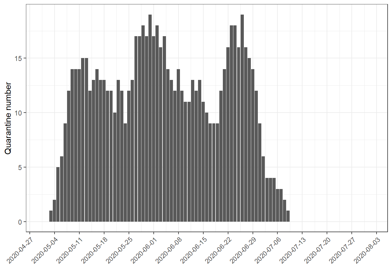
A more complete and complex example with medication tables
We have seen at the beginning of this post a simple example of a merge between a medication table and a long table of visits, when there is one ongoing treatment per visit. Let’s see now a more real example:
set.seed(123)
medication3 <- data.table(ID = c(1,1,1,1,2,2,2,3,3,3),
           medication = c("bio1","bio2","CSDMARD1","CSDMARD2","bio1","CSDMARD1","CSDMARD2","bio1","bio2","CSDMARD1"),
           start_date = ymd(c("2003-03-25","2006-04-27","2001-02-25","2005-01-04","2008-12-05","2006-07-25","2007-09-11",
                          "2004-06-03","2009-09-18","2002-01-01")),
           stop_date = ymd(c("2006-04-02",NA,NA,"2008-02-05","2010-07-12","2009-03-01","2012-08-01","2008-04-27",NA,NA)))

medication3
## ID medication start_date stop_date
## 1: 1 bio1 2003-03-25 2006-04-02
## 2: 1 bio2 2006-04-27 <NA>
## 3: 1 CSDMARD1 2001-02-25 <NA>
## 4: 1 CSDMARD2 2005-01-04 2008-02-05
## 5: 2 bio1 2008-12-05 2010-07-12
## 6: 2 CSDMARD1 2006-07-25 2009-03-01
## 7: 2 CSDMARD2 2007-09-11 2012-08-01
## 8: 3 bio1 2004-06-03 2008-04-27
## 9: 3 bio2 2009-09-18 <NA>
## 10: 3 CSDMARD1 2002-01-01 <NA>We have here:
- ongoing treatment, that are without stop dates
- biological unique treatments (i.e. the patient cannot have two biological treatment at the same time, so we want to have them in the same variable)
- situation were the patients have two or more treatments, which is common for example for conventional synthetic treatments (SCDMARDs)
I still want to have only one line per visit date in my long table. To be able to do the merge, I need to separate my medication table in 2 tables:
- Biological treatments, finished and ongoing
- SCDMARD, finished and ongoing
medication3[,start_date_merge := start_date]
medication3[,stop_date_merge := stop_date]
biotable <- medication3[medication %like% "bio"]
CSDMARDtable <- medication3[medication %like% "CSDMARD"]
I first start with the biological treatments. I need to consider two situations: the situation where the treatments are finished:
biotable[visit,on = .(ID,start_date_merge < visit.date,stop_date_merge > visit.date)] %>%
  head()
## ID medication start_date stop_date start_date_merge stop_date_merge
## 1: 1 bio1 2003-03-25 2006-04-02 2003-07-14 2003-07-14
## 2: 1 bio1 2003-03-25 2006-04-02 2004-06-09 2004-06-09
## 3: 1 bio1 2003-03-25 2006-04-02 2006-02-15 2006-02-15
## 4: 1 <NA> <NA> <NA> 2006-06-06 2006-06-06
## 5: 1 <NA> <NA> <NA> 2008-01-16 2008-01-16
## 6: 1 <NA> <NA> <NA> 2009-02-04 2009-02-04
## some_hosp_measure
## 1: 7.723726
## 2: 6.626613
## 3: 9.876177
## 4: 14.337912
## 5: 11.643162
## 6: 7.947991and situation where the treatment is ongoing:
biotable[is.na(stop_date)][visit,on = .(ID,start_date_merge < visit.date)]%>%
  head()
## ID medication start_date stop_date start_date_merge stop_date_merge
## 1: 1 <NA> <NA> <NA> 2003-07-14 <NA>
## 2: 1 <NA> <NA> <NA> 2004-06-09 <NA>
## 3: 1 <NA> <NA> <NA> 2006-02-15 <NA>
## 4: 1 bio2 2006-04-27 <NA> 2006-06-06 <NA>
## 5: 1 bio2 2006-04-27 <NA> 2008-01-16 <NA>
## 6: 1 bio2 2006-04-27 <NA> 2009-02-04 <NA>
## some_hosp_measure
## 1: 7.723726
## 2: 6.626613
## 3: 9.876177
## 4: 14.337912
## 5: 11.643162
## 6: 7.947991As we know that patient cannot have two treatments at the same time, we can just bind these two merged table:
bio_t <- rbind(biotable[visit,on = .(ID,start_date_merge < visit.date,stop_date_merge > visit.date)][!is.na(medication)],
               biotable[is.na(stop_date)][visit,on = .(ID,start_date_merge < visit.date)][!is.na(medication)])
setnames(bio_t,"start_date_merge","visit.date")
bio_t[,stop_date_merge := NULL]
head(bio_t)
## ID medication start_date stop_date visit.date some_hosp_measure
## 1: 1 bio1 2003-03-25 2006-04-02 2003-07-14 7.723726
## 2: 1 bio1 2003-03-25 2006-04-02 2004-06-09 6.626613
## 3: 1 bio1 2003-03-25 2006-04-02 2006-02-15 9.876177
## 4: 2 bio1 2008-12-05 2010-07-12 2010-04-03 12.507630
## 5: 3 bio1 2004-06-03 2008-04-27 2005-10-13 9.564050
## 6: 3 bio1 2004-06-03 2008-04-27 2006-10-10 10.306746and add the missing visit (i.e. the visits without any ongoign biological treatment)
visit2 <- merge(bio_t[,-"some_hosp_measure"],visit,all.y = T,by = c("ID","visit.date"))
visit2
## ID visit.date medication start_date stop_date some_hosp_measure
## 1: 1 2003-07-14 bio1 2003-03-25 2006-04-02 7.723726
## 2: 1 2004-06-09 bio1 2003-03-25 2006-04-02 6.626613
## 3: 1 2006-02-15 bio1 2003-03-25 2006-04-02 9.876177
## 4: 1 2006-06-06 bio2 2006-04-27 <NA> 14.337912
## 5: 1 2008-01-16 bio2 2006-04-27 <NA> 11.643162
## 6: 1 2009-02-04 bio2 2006-04-27 <NA> 7.947991
## 7: 1 2009-09-28 bio2 2006-04-27 <NA> 10.995701
## 8: 1 2009-11-15 bio2 2006-04-27 <NA> 9.054417
## 9: 1 2011-03-05 bio2 2006-04-27 <NA> 9.409857
## 10: 1 2012-03-24 bio2 2006-04-27 <NA> 8.610586
## 11: 2 2004-10-26 <NA> <NA> <NA> 11.675574
## 12: 2 2005-08-10 <NA> <NA> <NA> 12.415924
## 13: 2 2005-10-07 <NA> <NA> <NA> 9.388075
## 14: 2 2005-11-03 <NA> <NA> <NA> 7.864353
## 15: 2 2006-01-19 <NA> <NA> <NA> 9.584165
## 16: 2 2006-06-21 <NA> <NA> <NA> 6.066766
## 17: 2 2007-06-15 <NA> <NA> <NA> 11.790251
## 18: 2 2010-04-03 bio1 2008-12-05 2010-07-12 12.507630
## 19: 2 2010-07-19 <NA> <NA> <NA> 11.377281
## 20: 2 2012-06-07 <NA> <NA> <NA> 8.542218
## 21: 3 2003-12-14 <NA> <NA> <NA> 11.402712
## 22: 3 2005-10-13 bio1 2004-06-03 2008-04-27 9.564050
## 23: 3 2006-10-10 bio1 2004-06-03 2008-04-27 10.306746
## 24: 3 2006-12-20 bio1 2004-06-03 2008-04-27 9.239058
## 25: 3 2007-07-31 bio1 2004-06-03 2008-04-27 7.469207
## 26: 3 2007-11-25 bio1 2004-06-03 2008-04-27 7.753783
## 27: 3 2008-07-05 <NA> <NA> <NA> 8.749921
## 28: 3 2008-09-04 <NA> <NA> <NA> 11.756267
## 29: 3 2010-01-10 bio2 2009-09-18 <NA> 11.107835
## 30: 3 2010-11-27 bio2 2009-09-18 <NA> 10.852928
## ID visit.date medication start_date stop_date some_hosp_measureNow for the CSDMARD, as I can have several treatments at the same time, I will create a column per CSDMARD indicating if the patient is under this treatment at the given visit. Here an example for CSDMARD1 having a finished date:
CSDMARDtable[medication == "CSDMARD1"][
  visit[,-"some_hosp_measure"],on = .(ID,start_date_merge < visit.date,stop_date_merge > visit.date)][
    !is.na(medication),.(ID,visit.date = start_date_merge,CSDMARD1 = 1)]
## ID visit.date CSDMARD1
## 1: 2 2007-06-15 1The same for ongoing treatment, i.e. with missing stop dates:
CSDMARDtable[medication == "CSDMARD1" & is.na(stop_date)][
  visit[,-"some_hosp_measure"],on = .(ID,start_date_merge < visit.date)][
    !is.na(medication),.(ID,visit.date = start_date_merge,CSDMARD1 = 1)]
## ID visit.date CSDMARD1
## 1: 1 2003-07-14 1
## 2: 1 2004-06-09 1
## 3: 1 2006-02-15 1
## 4: 1 2006-06-06 1
## 5: 1 2008-01-16 1
## 6: 1 2009-02-04 1
## 7: 1 2009-09-28 1
## 8: 1 2009-11-15 1
## 9: 1 2011-03-05 1
## 10: 1 2012-03-24 1
## 11: 3 2003-12-14 1
## 12: 3 2005-10-13 1
## 13: 3 2006-10-10 1
## 14: 3 2006-12-20 1
## 15: 3 2007-07-31 1
## 16: 3 2007-11-25 1
## 17: 3 2008-07-05 1
## 18: 3 2008-09-04 1
## 19: 3 2010-01-10 1
## 20: 3 2010-11-27 1If now repeat these two steps in a loop for the different CSDMARDs:
tmp <- lapply(unique(CSDMARDtable$medication),function(x){
  rbind(
    CSDMARDtable[medication == x][
  visit[,-"some_hosp_measure"],on = .(ID,start_date_merge < visit.date,stop_date_merge > visit.date)][
    !is.na(medication),setNames(.(ID,start_date_merge,1),c("ID","visit.date",x))  ],
    CSDMARDtable[medication == x & is.na(stop_date)][
  visit[,-"some_hosp_measure"],on = .(ID,start_date_merge < visit.date)][
    !is.na(medication),setNames(.(ID,start_date_merge,1),c("ID","visit.date",x)) ]
  )
})
To then merge everything together:
tmp[[length(tmp)+1]] <- visit2
final <- Reduce(
  function(x,y) merge(x,y,all = T,by = c("visit.date","ID")),
  tmp
)
setkeyv(final,c("ID","visit.date"))
final
## visit.date ID CSDMARD1 CSDMARD2 medication start_date stop_date
## 1: 2003-07-14 1 1 NA bio1 2003-03-25 2006-04-02
## 2: 2004-06-09 1 1 NA bio1 2003-03-25 2006-04-02
## 3: 2006-02-15 1 1 1 bio1 2003-03-25 2006-04-02
## 4: 2006-06-06 1 1 1 bio2 2006-04-27 <NA>
## 5: 2008-01-16 1 1 1 bio2 2006-04-27 <NA>
## 6: 2009-02-04 1 1 NA bio2 2006-04-27 <NA>
## 7: 2009-09-28 1 1 NA bio2 2006-04-27 <NA>
## 8: 2009-11-15 1 1 NA bio2 2006-04-27 <NA>
## 9: 2011-03-05 1 1 NA bio2 2006-04-27 <NA>
## 10: 2012-03-24 1 1 NA bio2 2006-04-27 <NA>
## 11: 2004-10-26 2 NA NA <NA> <NA> <NA>
## 12: 2005-08-10 2 NA NA <NA> <NA> <NA>
## 13: 2005-10-07 2 NA NA <NA> <NA> <NA>
## 14: 2005-11-03 2 NA NA <NA> <NA> <NA>
## 15: 2006-01-19 2 NA NA <NA> <NA> <NA>
## 16: 2006-06-21 2 NA NA <NA> <NA> <NA>
## 17: 2007-06-15 2 1 NA <NA> <NA> <NA>
## 18: 2010-04-03 2 NA 1 bio1 2008-12-05 2010-07-12
## 19: 2010-07-19 2 NA 1 <NA> <NA> <NA>
## 20: 2012-06-07 2 NA 1 <NA> <NA> <NA>
## 21: 2003-12-14 3 1 NA <NA> <NA> <NA>
## 22: 2005-10-13 3 1 NA bio1 2004-06-03 2008-04-27
## 23: 2006-10-10 3 1 NA bio1 2004-06-03 2008-04-27
## 24: 2006-12-20 3 1 NA bio1 2004-06-03 2008-04-27
## 25: 2007-07-31 3 1 NA bio1 2004-06-03 2008-04-27
## 26: 2007-11-25 3 1 NA bio1 2004-06-03 2008-04-27
## 27: 2008-07-05 3 1 NA <NA> <NA> <NA>
## 28: 2008-09-04 3 1 NA <NA> <NA> <NA>
## 29: 2010-01-10 3 1 NA bio2 2009-09-18 <NA>
## 30: 2010-11-27 3 1 NA bio2 2009-09-18 <NA>
## visit.date ID CSDMARD1 CSDMARD2 medication start_date stop_date
## some_hosp_measure
## 1: 7.723726
## 2: 6.626613
## 3: 9.876177
## 4: 14.337912
## 5: 11.643162
## 6: 7.947991
## 7: 10.995701
## 8: 9.054417
## 9: 9.409857
## 10: 8.610586
## 11: 11.675574
## 12: 12.415924
## 13: 9.388075
## 14: 7.864353
## 15: 9.584165
## 16: 6.066766
## 17: 11.790251
## 18: 12.507630
## 19: 11.377281
## 20: 8.542218
## 21: 11.402712
## 22: 9.564050
## 23: 10.306746
## 24: 9.239058
## 25: 7.469207
## 26: 7.753783
## 27: 8.749921
## 28: 11.756267
## 29: 11.107835
## 30: 10.852928
## some_hosp_measureEt voilà!
Here are two example in stackoverflow where I proposed a solution with non equi joins.